Estimating a PEM survival model with Gamma baseline hazard
In [ ]:
%load_ext autoreload
%autoreload 2
%matplotlib inline
import random
random.seed(1100038344)
import survivalstan
import numpy as np
import pandas as pd
from stancache import stancache
from matplotlib import pyplot as plt
In [2]:
print(survivalstan.models.pem_survival_model_gamma)
/*  Variable naming:
 // dimensions
 N          = total number of observations (length of data)
 S          = number of sample ids
 T          = max timepoint (number of timepoint ids)
 M          = number of covariates

 // data
 s          = sample id for each obs
 t          = timepoint id for each obs
 event      = integer indicating if there was an event at time t for sample s
 x          = matrix of real-valued covariates at time t for sample n [N, X]
 obs_t      = observed end time for interval for timepoint for that obs

*/
// Jacqueline Buros Novik <jackinovik@gmail.com>


data {
  int<lower=1> N;
  int<lower=1> S;
  int<lower=1> T;
  int<lower=0> M;
  int<lower=1, upper=N> s[N];     // sample id
  int<lower=1, upper=T> t[N];     // timepoint id
  int<lower=0, upper=1> event[N]; // 1: event, 0:censor
  matrix[N, M] x;                 // explanatory vars
  real<lower=0> obs_t[N];         // observed end time for each obs
  real<lower=0> t_dur[T];
  real<lower=0> t_obs[T];
}
transformed data {
  real c_unit;
  real r_unit;
  int n_trans[S, T];

  // scale for baseline hazard params (fixed)
  c_unit = 0.001;
  r_unit = 0.1;

  // n_trans used to map each sample*timepoint to n (used in gen quantities)
  // map each patient/timepoint combination to n values
  for (n in 1:N) {
      n_trans[s[n], t[n]] = n;
  }

  // fill in missing values with n for max t for that patient
  // ie assume "last observed" state applies forward (may be problematic for TVC)
  // this allows us to predict failure times >= observed survival times
  for (samp in 1:S) {
      int last_value;
      last_value = 0;
      for (tp in 1:T) {
          // manual says ints are initialized to neg values
          // so <=0 is a shorthand for "unassigned"
          if (n_trans[samp, tp] <= 0 && last_value != 0) {
              n_trans[samp, tp] = last_value;
          } else {
              last_value = n_trans[samp, tp];
          }
      }
  }
}
parameters {
  vector<lower=0>[T] baseline; // unstructured baseline hazard for each timepoint t
  vector[M] beta; // beta for each covariate
  real<lower=0> c_raw;
  real<lower=0> r_raw;
}
transformed parameters {
  vector[N] log_hazard;
  vector[T] log_baseline;
  real<lower=0> c;
  real<lower=0> r;


  log_baseline = log(baseline);

  r = r_unit*r_raw;
  c = c_unit*c_raw;

  for (n in 1:N) {
    log_hazard[n] = x[n,]*beta + log_baseline[t[n]];
  }
}
model {
  for (i in 1:T) {
      baseline[i] ~ gamma(r * t_dur[i] * c, c);
  }
  beta ~ cauchy(0, 2);
  event ~ poisson_log(log_hazard);
  c_raw ~ normal(0, 1);
  r_raw ~ normal(0, 1);
}
generated quantities {
  real log_lik[N];
  int y_hat_mat[S, T]; // ppcheck for each S*T combination
  real y_hat_time[S];       // predicted failure time for each sample
  int y_hat_event[S];      // predicted event (0:censor, 1:event)

  // log-likelihood, for loo
  for (n in 1:N) {
      log_lik[n] = poisson_log_lpmf(event[n] | log_hazard[n]);
  }

  // posterior predicted values
  for (samp in 1:S) {
      int sample_alive;
      sample_alive = 1;
      for (tp in 1:T) {
        if (sample_alive == 1) {
              real log_haz;
              int n;
              int pred_y;

              // determine predicted value of y
              n = n_trans[samp, tp];
              log_haz = x[n,]*beta + log_baseline[tp];
              if (log_haz < log(pow(2, 30)))
                  pred_y = poisson_log_rng(log_haz);
              else
                  pred_y = 9;

              // mark this patient as ineligible for future tps
              // note: deliberately make 9s ineligible
              if (pred_y >= 1) {
                  sample_alive = 0;
                  y_hat_time[samp] = t_obs[tp];
                  y_hat_event[samp] = 1;
              }

              // save predicted value of y to matrix
              y_hat_mat[samp, tp] = pred_y;
          }
          else if (sample_alive == 0) {
              y_hat_mat[samp, tp] = 9;
          }
      } // end per-timepoint loop

      // if patient still alive at max
      //
      if (sample_alive == 1) {
          y_hat_time[samp] = t_obs[T];
          y_hat_event[samp] = 0;
      }
  } // end per-sample loop
}
In [3]:
d = stancache.cached(
    survivalstan.sim.sim_data_exp_correlated,
    N=100,
    censor_time=20,
    rate_form='1 + sex',
    rate_coefs=[-3, 0.5],
)
d['age_centered'] = d['age'] - d['age'].mean()
d.head()
INFO:stancache.stancache:sim_data_exp_correlated: cache_filename set to sim_data_exp_correlated.cached.N_100.censor_time_20.rate_coefs_54462717316.rate_form_1 + sex.pkl
INFO:stancache.stancache:sim_data_exp_correlated: Loading result from cache
Out[3]:
| age | sex | rate | true_t | t | event | index | age_centered | |
|---|---|---|---|---|---|---|---|---|
| 0 | 59 | male | 0.082085 | 20.948771 | 20.000000 | False | 0 | 4.18 |
| 1 | 58 | male | 0.082085 | 12.827519 | 12.827519 | True | 1 | 3.18 |
| 2 | 61 | female | 0.049787 | 27.018886 | 20.000000 | False | 2 | 6.18 |
| 3 | 57 | female | 0.049787 | 62.220296 | 20.000000 | False | 3 | 2.18 |
| 4 | 55 | male | 0.082085 | 10.462045 | 10.462045 | True | 4 | 0.18 |
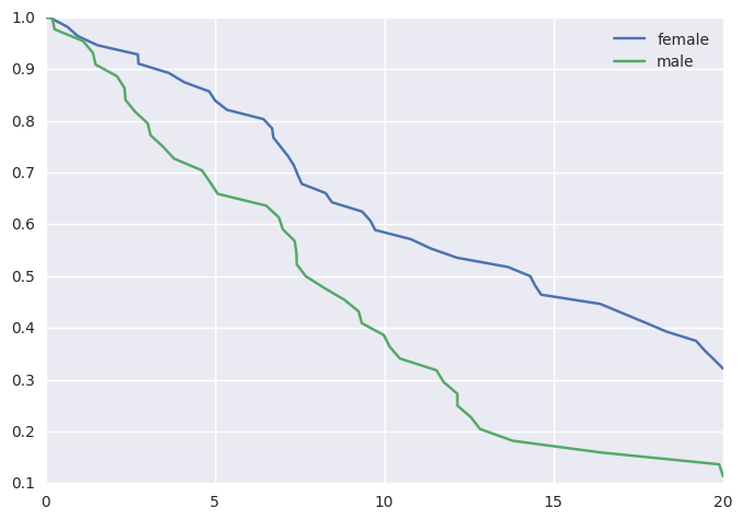
In [4]:
survivalstan.utils.plot_observed_survival(df=d[d['sex']=='female'], event_col='event', time_col='t', label='female')
survivalstan.utils.plot_observed_survival(df=d[d['sex']=='male'], event_col='event', time_col='t', label='male')
plt.legend()
Out[4]:
<matplotlib.legend.Legend at 0x7f9fac008eb8>
In [5]:
dlong = stancache.cached(
    survivalstan.prep_data_long_surv,
    df=d, event_col='event', time_col='t'
)
INFO:stancache.stancache:prep_data_long_surv: cache_filename set to prep_data_long_surv.cached.df_33772694934.event_col_event.time_col_t.pkl
INFO:stancache.stancache:prep_data_long_surv: Loading result from cache
In [6]:
dlong.head()
Out[6]:
| age | sex | rate | true_t | t | event | index | age_centered | key | end_time | end_failure | |
|---|---|---|---|---|---|---|---|---|---|---|---|
| 0 | 59 | male | 0.082085 | 20.948771 | 20.0 | False | 0 | 4.18 | 1 | 20.000000 | False |
| 1 | 59 | male | 0.082085 | 20.948771 | 20.0 | False | 0 | 4.18 | 1 | 12.827519 | False |
| 2 | 59 | male | 0.082085 | 20.948771 | 20.0 | False | 0 | 4.18 | 1 | 10.462045 | False |
| 3 | 59 | male | 0.082085 | 20.948771 | 20.0 | False | 0 | 4.18 | 1 | 0.196923 | False |
| 4 | 59 | male | 0.082085 | 20.948771 | 20.0 | False | 0 | 4.18 | 1 | 9.244121 | False |
In [7]:
testfit = survivalstan.fit_stan_survival_model(
    model_cohort = 'test model',
    model_code = survivalstan.models.pem_survival_model_gamma,
    df = dlong,
    sample_col = 'index',
    timepoint_end_col = 'end_time',
    event_col = 'end_failure',
    formula = '~ age_centered + sex',
    iter = 5000,
    chains = 4,
    seed = 9001,
    FIT_FUN = stancache.cached_stan_fit,
    )
INFO:stancache.stancache:Step 1: Get compiled model code, possibly from cache
INFO:stancache.stancache:StanModel: cache_filename set to anon_model.cython_0_25_1.model_code_72990130769.pystan_2_12_0_0.stanmodel.pkl
INFO:stancache.stancache:StanModel: Loading result from cache
INFO:stancache.stancache:Step 2: Get posterior draws from model, possibly from cache
INFO:stancache.stancache:sampling: cache_filename set to anon_model.cython_0_25_1.model_code_72990130769.pystan_2_12_0_0.stanfit.chains_4.data_64545635565.iter_5000.seed_9001.pkl
INFO:stancache.stancache:sampling: Starting execution
INFO:stancache.stancache:sampling: Execution completed (0:02:26.153391 elapsed)
INFO:stancache.stancache:sampling: Saving results to cache
/home/jacquelineburos/miniconda3/envs/python3/lib/python3.5/site-packages/stancache/stancache.py:251: UserWarning: Pickling fit objects is an experimental feature!
The relevant StanModel instance must be pickled along with this fit object.
When unpickling the StanModel must be unpickled first.
  pickle.dump(res, open(cache_filepath, 'wb'), pickle.HIGHEST_PROTOCOL)
/home/jacquelineburos/miniconda3/envs/python3/lib/python3.5/site-packages/stanity/psis.py:228: FutureWarning: elementwise comparison failed; returning scalar instead, but in the future will perform elementwise comparison
  elif sort == 'in-place':
/home/jacquelineburos/miniconda3/envs/python3/lib/python3.5/site-packages/stanity/psis.py:246: VisibleDeprecationWarning: using a non-integer number instead of an integer will result in an error in the future
  bs /= 3 * x[sort[np.floor(n/4 + 0.5) - 1]]
/home/jacquelineburos/miniconda3/envs/python3/lib/python3.5/site-packages/stanity/psis.py:262: RuntimeWarning: overflow encountered in exp
  np.exp(temp, out=temp)
/home/jacquelineburos/miniconda3/envs/python3/lib/python3.5/site-packages/stanity/psis.py:246: RuntimeWarning: divide by zero encountered in true_divide
  bs /= 3 * x[sort[np.floor(n/4 + 0.5) - 1]]
/home/jacquelineburos/miniconda3/envs/python3/lib/python3.5/site-packages/stanity/psis.py:250: RuntimeWarning: invalid value encountered in multiply
  temp = ks[:,None] * x
/home/jacquelineburos/miniconda3/envs/python3/lib/python3.5/site-packages/stanity/psis.py:267: RuntimeWarning: invalid value encountered in greater_equal
  dii = w >= 10 * np.finfo(float).eps
/home/jacquelineburos/miniconda3/envs/python3/lib/python3.5/site-packages/stanity/psis.py:282: RuntimeWarning: invalid value encountered in double_scalars
  sigma = -k / b
In [8]:
survivalstan.utils.print_stan_summary([testfit], pars='lp__')
            mean  se_mean        sd         2.5%          50%       97.5%      Rhat
lp__ -1034.96497  0.18312  7.354494 -1050.563484 -1034.543604 -1021.53023  1.000819
In [9]:
survivalstan.utils.print_stan_summary([testfit], pars='log_baseline')
                        mean   se_mean          sd        2.5%         50%      97.5%      Rhat
log_baseline[0]    -5.540533  0.026349    1.317162   -8.741271   -5.317482  -3.605955  1.000660
log_baseline[1]    -5.540373  0.026410    1.312295   -8.765512   -5.305697  -3.661229  1.000160
log_baseline[2]    -5.533987  0.025182    1.277367   -8.563403   -5.341926  -3.613802  1.000899
log_baseline[3]    -5.499061  0.023197    1.266738   -8.526801   -5.300919  -3.598318  1.000996
log_baseline[4]    -5.529027  0.029142    1.376488   -8.883094   -5.280803  -3.553426  1.001002
log_baseline[5]    -5.471047  0.025521    1.260655   -8.429872   -5.272214  -3.596805  1.002028
log_baseline[6]    -5.499416  0.034998    1.321609   -8.548750   -5.291451  -3.584369  1.003210
log_baseline[7]    -5.464198  0.024734    1.288292   -8.466082   -5.228081  -3.575405  1.000619
log_baseline[8]    -5.466310  0.027385    1.284197   -8.583571   -5.262634  -3.536853  1.001117
log_baseline[9]    -5.416356  0.024357    1.279819   -8.469762   -5.221550  -3.528211  1.001357
log_baseline[10]   -5.440701  0.027773    1.306535   -8.676018   -5.228972  -3.541475  1.001608
log_baseline[11]   -5.434051  0.027698    1.305317   -8.664646   -5.225114  -3.512998  0.999949
log_baseline[12]   -5.370823  0.028533    1.284318   -8.459077   -5.161179  -3.454565  1.001136
log_baseline[13]   -5.393917  0.024404    1.280480   -8.626593   -5.192589  -3.486274  1.000423
log_baseline[14]   -5.364330  0.025443    1.273700   -8.327442   -5.166064  -3.490194  1.002779
log_baseline[15]   -5.357747  0.025662    1.282847   -8.510490   -5.145634  -3.463617  1.002548
log_baseline[16]   -5.378575  0.027974    1.302219   -8.521636   -5.152384  -3.489239  1.003528
log_baseline[17]   -5.295181  0.026170    1.249062   -8.246395   -5.115480  -3.442103  1.004022
log_baseline[18]   -5.346658  0.027128    1.301594   -8.462238   -5.129009  -3.403453  1.002558
log_baseline[19]   -5.293308  0.027616    1.280204   -8.270132   -5.103891  -3.405552  1.000711
log_baseline[20]   -5.312085  0.024626    1.318119   -8.478142   -5.086743  -3.394770  1.000745
log_baseline[21]   -5.277845  0.026557    1.264723   -8.303782   -5.068627  -3.349496  1.000715
log_baseline[22]   -5.306103  0.027747    1.309989   -8.480791   -5.098819  -3.372876  1.002474
log_baseline[23]   -5.240126  0.024418    1.274211   -8.374662   -5.031179  -3.368183  1.002631
log_baseline[24]   -5.180366  0.023456    1.229393   -8.199401   -4.991827  -3.339248  1.002037
log_baseline[25]   -5.220781  0.025189    1.279213   -8.155421   -5.026628  -3.347359  0.999862
log_baseline[26]   -5.198388  0.027133    1.293306   -8.334439   -4.988685  -3.310959  1.002848
log_baseline[27]   -5.145882  0.024486    1.269478   -8.201074   -4.960108  -3.261169  1.000358
log_baseline[28]   -5.112184  0.023308    1.235079   -8.159944   -4.913842  -3.245869  1.001038
log_baseline[29]   -5.130311  0.028653    1.303939   -8.381742   -4.914959  -3.271805  1.001287
log_baseline[30]   -5.197454  0.026676    1.342558   -8.362530   -4.956216  -3.213312  1.000961
log_baseline[31]   -5.188365  0.027795    1.344816   -8.474813   -4.969168  -3.277665  1.002005
log_baseline[32]   -5.102617  0.024780    1.260118   -8.178528   -4.901117  -3.213594  1.000780
log_baseline[33]   -5.075221  0.024387    1.227845   -7.991722   -4.885576  -3.214388  1.000436
log_baseline[34]   -5.110409  0.029528    1.336298   -8.447845   -4.872393  -3.193095  1.001111
log_baseline[35]   -5.031990  0.024814    1.248103   -8.051273   -4.841412  -3.165030  1.000698
log_baseline[36]   -5.050843  0.025298    1.288200   -8.189802   -4.835042  -3.140867  1.002413
log_baseline[37]   -5.027862  0.025181    1.274591   -7.993631   -4.829429  -3.130617  1.002734
log_baseline[38]   -5.043253  0.031843    1.332076   -8.392334   -4.800582  -3.117772  1.001792
log_baseline[39]   -5.009148  0.027024    1.286125   -8.114673   -4.801411  -3.083061  1.001948
log_baseline[40]   -4.977261  0.022727    1.253310   -8.021432   -4.786938  -3.099191  1.000618
log_baseline[41]   -4.973488  0.026404    1.297564   -8.165326   -4.762586  -3.063354  1.000620
log_baseline[42]   -4.976570  0.026160    1.289808   -8.134780   -4.785349  -3.061472  1.000685
log_baseline[43]   -4.919019  0.025599    1.277389   -8.050034   -4.700221  -3.016657  1.001715
log_baseline[44]   -4.900334  0.025927    1.293227   -8.049396   -4.679596  -2.980225  1.000656
log_baseline[45]   -4.907134  0.025745    1.276647   -8.046290   -4.690973  -3.021486  1.001499
log_baseline[46]   -4.855415  0.023345    1.255215   -7.826891   -4.654950  -2.972896  1.001151
log_baseline[47]   -4.832234  0.021958    1.254851   -7.809152   -4.639160  -2.926565  1.001058
log_baseline[48]   -4.798222  0.024395    1.255120   -7.870438   -4.580276  -2.924569  1.000580
log_baseline[49]   -4.838834  0.029046    1.346472   -8.135627   -4.612250  -2.866454  1.001520
log_baseline[50]   -4.760367  0.024182    1.265330   -7.845615   -4.552539  -2.875869  1.000354
log_baseline[51]   -4.737922  0.024380    1.249825   -7.791359   -4.524863  -2.860117  1.000065
log_baseline[52]   -4.751358  0.028862    1.327670   -8.044268   -4.540209  -2.862803  1.000918
log_baseline[53]   -4.685420  0.023722    1.284065   -7.852333   -4.469523  -2.795754  1.001032
log_baseline[54]   -4.695464  0.025316    1.294588   -7.810316   -4.503222  -2.782197  1.000505
log_baseline[55]   -4.662545  0.027774    1.317164   -7.848580   -4.440736  -2.771303  1.000641
log_baseline[56]   -4.669330  0.030262    1.321870   -7.914412   -4.434960  -2.743924  1.000618
log_baseline[57]   -4.620962  0.025575    1.282324   -7.585949   -4.400851  -2.737336  1.003473
log_baseline[58]   -4.564812  0.025214    1.287904   -7.671804   -4.338766  -2.704413  1.001306
log_baseline[59]   -4.562128  0.030414    1.350609   -7.910983   -4.324704  -2.648129  1.000886
log_baseline[60]   -4.542367  0.032122    1.338757   -7.768437   -4.320009  -2.624694  1.002409
log_baseline[61]   -4.480764  0.025349    1.287803   -7.550987   -4.280852  -2.593134  1.001754
log_baseline[62]   -4.430831  0.024307    1.228657   -7.382741   -4.239083  -2.589439  1.001206
log_baseline[63]   -4.395725  0.023673    1.273268   -7.384986   -4.209973  -2.479231  1.000442
log_baseline[64]   -4.346682  0.025621    1.266635   -7.426116   -4.141308  -2.442702  1.002046
log_baseline[65]   -4.312951  0.024879    1.298957   -7.481565   -4.094432  -2.411871  1.001782
log_baseline[66]   -4.272058  0.023535    1.271993   -7.300271   -4.066569  -2.414926  1.001380
log_baseline[67]   -4.278248  0.024941    1.301696   -7.406780   -4.063855  -2.381025  1.001246
log_baseline[68]   -4.239232  0.022731    1.255980   -7.282352   -4.042431  -2.363243  1.000641
log_baseline[69]   -4.220383  0.023864    1.257355   -7.227408   -4.033891  -2.300163  1.000607
log_baseline[70]   -4.174461  0.033438    1.387179   -7.389505   -3.925402  -2.265936  1.002038
log_baseline[71]   -4.090127  0.022568    1.252697   -7.085192   -3.892866  -2.207512  1.002348
log_baseline[72]   -4.110447  0.027878    1.315899   -7.399702   -3.860361  -2.205056  1.001732
log_baseline[73]   -4.056023  0.027877    1.311094   -7.247058   -3.837001  -2.137026  1.001115
log_baseline[74]   -4.023769  0.024615    1.255600   -7.067530   -3.820071  -2.142365  1.001948
log_baseline[75]   -4.049963  0.026498    1.295967   -7.201009   -3.854413  -2.140042  1.000684
log_baseline[76]   -4.047071  0.028314    1.357597   -7.297987   -3.803428  -2.082792  1.001065
log_baseline[77] -322.669893  5.131864  200.339993 -685.976286 -304.462026 -18.223910  1.002720
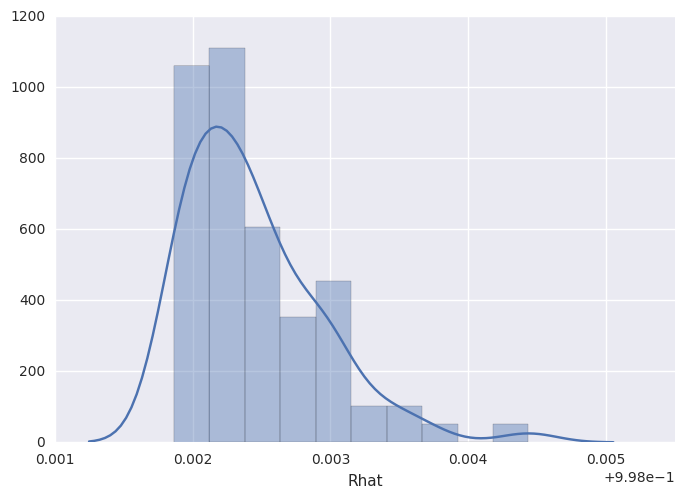
In [10]:
survivalstan.utils.plot_stan_summary([testfit], pars='baseline')
INFO:survivalstan.utils:Warning - 1 rows removed due to NaN values for Rhat. This may indicate a problem in your model estimation.
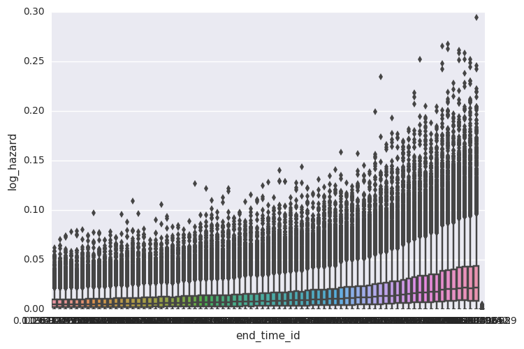
In [11]:
survivalstan.utils.plot_coefs([testfit], element='baseline')
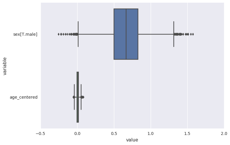
In [12]:
survivalstan.utils.plot_coefs([testfit])
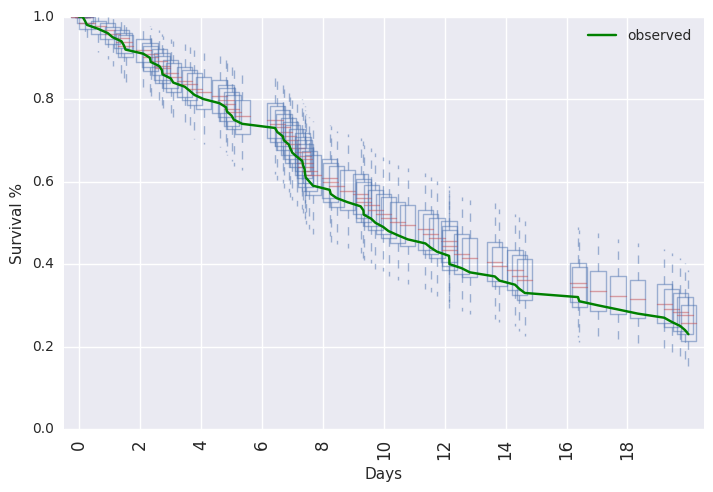
In [13]:
survivalstan.utils.plot_pp_survival([testfit], fill=False)
survivalstan.utils.plot_observed_survival(df=d, event_col='event', time_col='t', color='green', label='observed')
plt.legend()
Out[13]:
<matplotlib.legend.Legend at 0x7f9ec3bcba20>
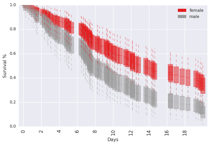
In [14]:
survivalstan.utils.plot_pp_survival([testfit], by='sex')
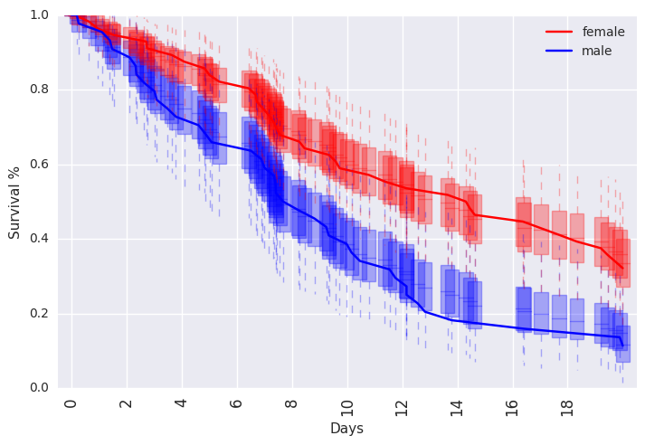
In [15]:
ppsurv = survivalstan.utils.prep_pp_survival_data([testfit], by='sex')
In [16]:
subplot = plt.subplots(1, 1)
survivalstan.utils._plot_pp_survival_data(ppsurv.query('sex == "male"').copy(),
                                          subplot=subplot, color='blue', alpha=0.3)
survivalstan.utils._plot_pp_survival_data(ppsurv.query('sex == "female"').copy(),
                                          subplot=subplot, color='red', alpha=0.3)
survivalstan.utils.plot_observed_survival(df=d[d['sex']=='female'], event_col='event', time_col='t',
                                          color='red', label='female')
survivalstan.utils.plot_observed_survival(df=d[d['sex']=='male'], event_col='event', time_col='t',
                                          color='blue', label='male')
plt.legend()
Out[16]:
<matplotlib.legend.Legend at 0x7f9f9714d7f0>
In [17]: